Plots bubble plot on map

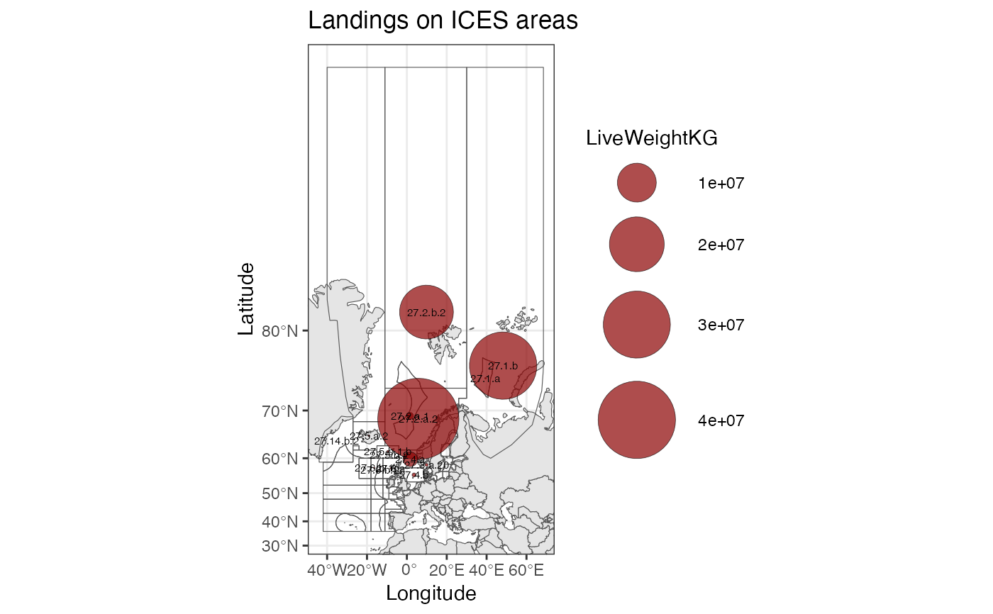
Plots scalar nonegative quantities associated with an area code, as bubbles on a map.

Usage

plotBubbleMap(
  data,
  areaCol,
  quantityCol,
  areaDef,
  areaNameCol = "StratumName",
  legendTitle = quantityCol,
  areaLabels = T,
  xlim = NULL,
  ylim = NULL,
  areaLabelSize = 2,
  bubbleColor = "darkred",
  bubbleSize = 10,
  bubbleShape = 21,
  title = "",
  projection = NULL
)

Arguments

data

data.frame with quantities to be plotted

areaCol

character() identifing column in 'data' that specify area codes, must correspond to 'areaNameCol'

quantityCol

character() identifing column in 'data' that specify quantities to be plotted

areaDef

SpatialPolygonsDataFrame

areaNameCol

identifies column in 'areaDef' with label names for the areas, must correspond to 'areaCol'

legendTitle

title for the legend (explains what the quantities are)

areaLabels

logical whether to plot area labels

xlim

x axis limits in degrees longitude

ylim

y axis limits in degrees latitude

areaLabelSize

size for any area labels

bubbleColor

color of the bubbles

bubbleSize

size for the bubbles

bubbleShape

shape of the "bubbles". Default to circle (21). Use e.g. 22 for squares (consult list of pch values)

title

plot title

projection

proj4string or EPSG code specifying the desired projection, see st_crs. Defaults to mercator projection

Details

The quantities (quantityCol) is aggregated (summed, ignoring NAs) over combinations of area and group ('areaCol' and 'groupCol') (if given) Bubble areas are proportional to the quantities.

Examples

 data(landings)
 data(ICESareas)
 plotBubbleMap(landings, "Area", "LiveWeightKG",
       areaDef = ICESareas, areaNameCol = "Area_Full",
       bubbleSize = 20, title="Landings on ICES areas")
#> Spherical geometry (s2) switched off
#> Spherical geometry (s2) switched on